
I sat down with Stephanie Chastain, CPE’s Excel Trainer, to learn more about Excel and its functionality. Stephanie brings a wealth of knowledge and expertise to CPE, having been an IT trainer for 25 years. Check out five helpful, time-saving Excel tips that Stephanie has found most students don’t know before starting Excel training.
TIP #1: USE THE AUTOFILL HANDLE TO AUTOMATICALLY NUMBER EACH LINE.
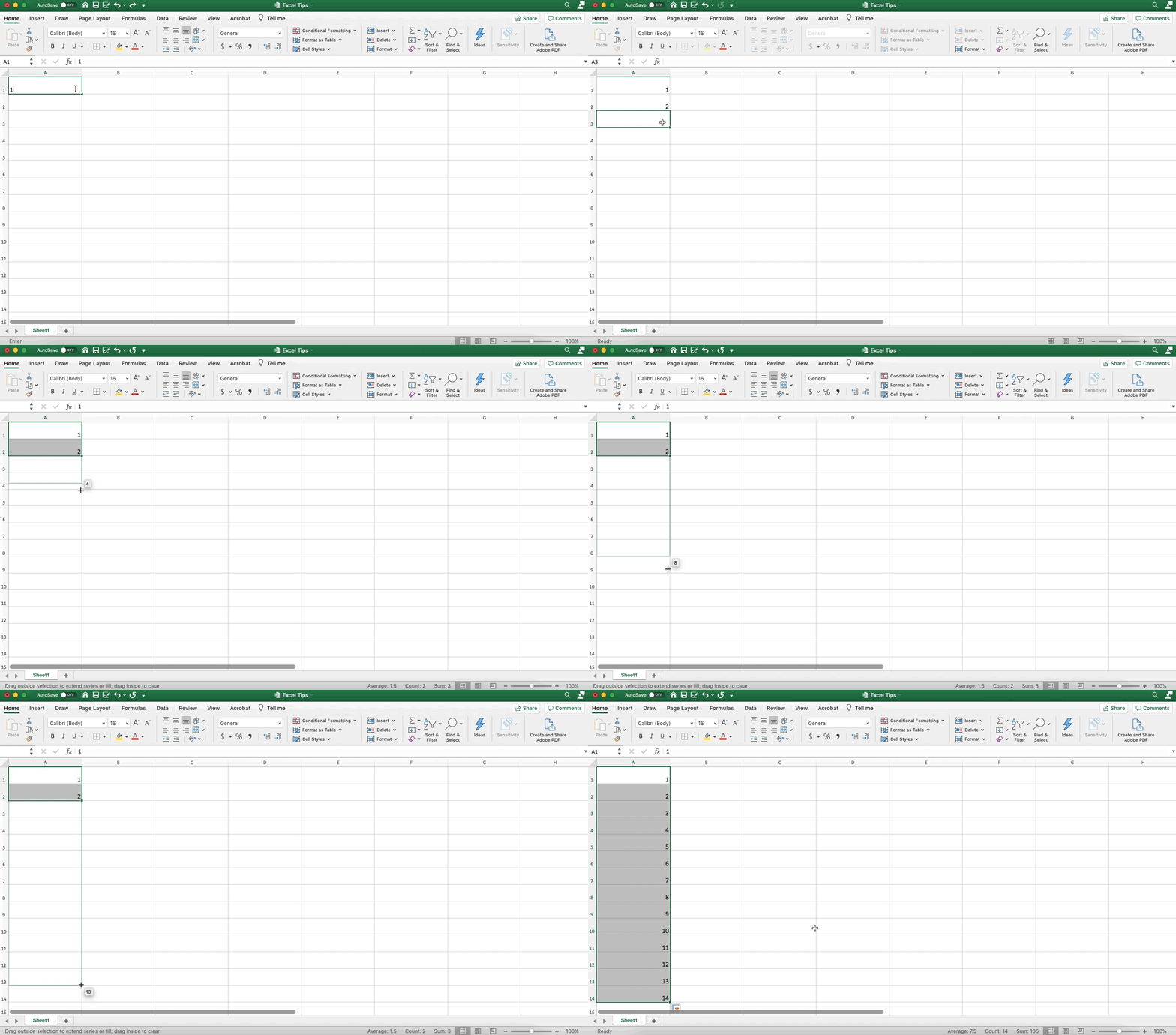
Excel is often used for numbering data. You can use the autofill handle to quickly populate cells with data without having to manually enter every piece of individual data. Let’s say you have to type in Line 1, Line 2, Line 3, etc. You would:
- Put in at least two numbers in the first two cells of data. There must be at least two numbers for the autofill handle to work.
- Highlight your series (the numbers you have entered in the cells).
- In the bottom right-hand corner of your series, hover your mouse over the square outline. A solid plus sign will pop up. Now, you can click and drag as far down as you want your data to be entered. Data in the same increments you have chosen (for example, the lines would continue in increments of 1) will be auto-filled into your cells.
Not only can the autofill handle be used for numbering, but it can be used for custom lists as well as with certain words using whatever nomenclature you use for abbreviations. It may not seem to be a giant time-saver at first, but using the handle for repetitive tasks will save you a ton of time in the long run.
TIP #2: HIGHLIGHT NUMBERS TO COMPUTE DATA QUICKLY.
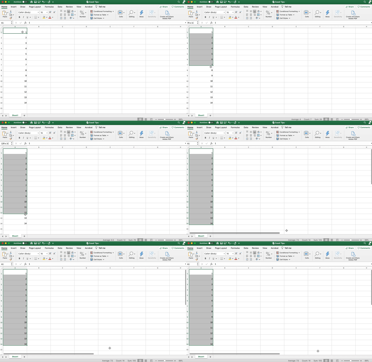
Not many people realize that you can quickly see the sum, average, and count of data at the bottom of your spreadsheet. These figures are located in what’s called the “status bar.” Instead of inserting a formula or function to give you this information, you would:
- Highlight the numbers you want to pull data for.
- Look at the “status bar” (located at the bottom of the Excel spreadsheet).
- See the sum, average, and count data you need.
Let’s say your boss calls you and asks, “Can you tell me how many entries we have this month in XYZ category?” You can use this method to quickly pull data.
TIP #3: INSERT MULTIPLE ROWS AND COLUMNS QUICKLY.
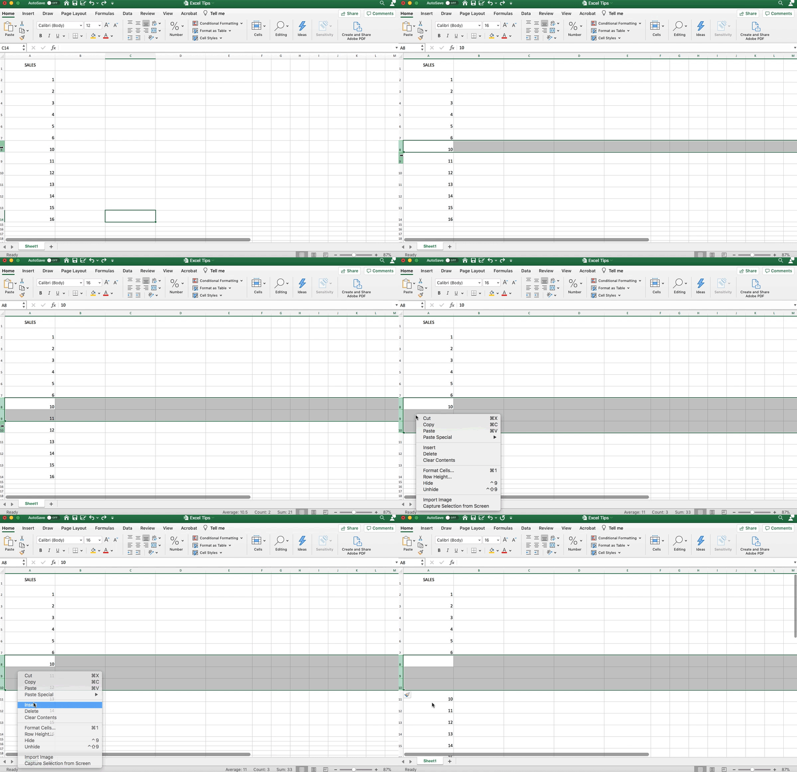
Instead of entering rows individually, you can quickly add multiple rows and columns to your spreadsheet. You would:
- Highlight the same number of columns (or rows) you would like to insert.
- Right-click your selection.
- Select Insert.
- The number of columns (or rows) you highlighted will be added. This is a very simple, yet effective time-saver!
TIP #4: RESIZE COLUMNS TO ACCOMMODATE VARIOUS DATA SIZES.
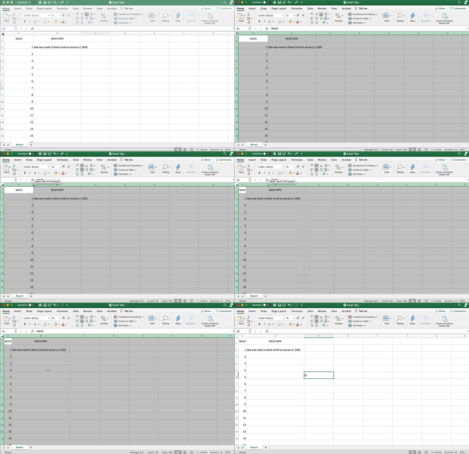
Excel users often make spreadsheets and resize individual columns to have data fit perfectly in each one. If you’re not worried about aesthetics, but just want to get as much data as possible on one page, there is a way to automatically resize every column at one time to match the largest set of data in a particular column. To quickly resize columns, you would:
- Click on the Select All button (in the top left corner, between sections A and 1, on your spreadsheet).
- Double-click between 2 columns to resize the entire spreadsheet.
You can apply the same steps to rows by clicking between 2 rows in the fourth step.
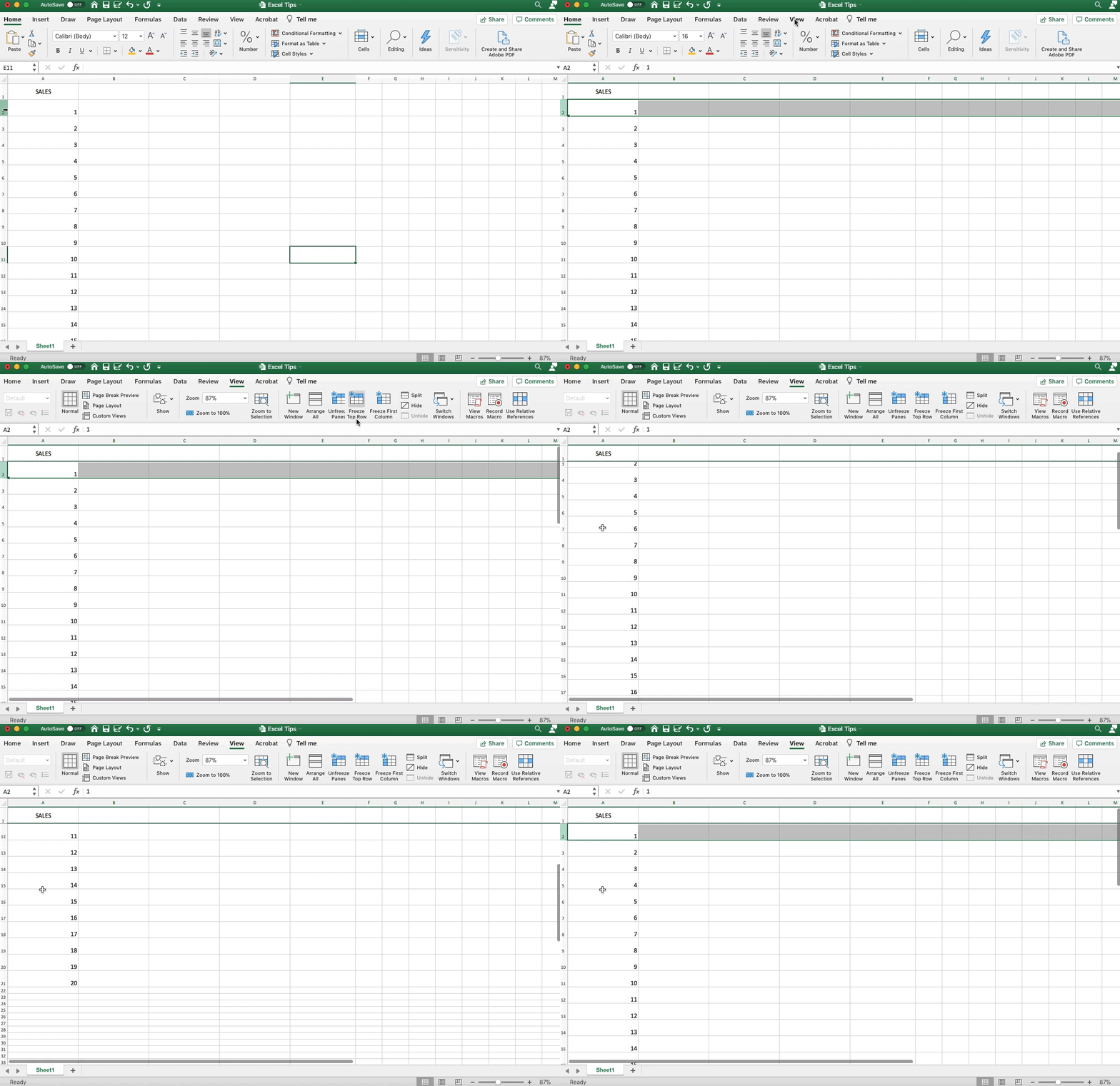
TIP #5: FREEZE HEADINGS USING THE FREEZE PANE FEATURE.
It’s easy to start scrolling and realize that you don’t even know what you’re looking at anymore. The freeze pane feature keeps your column headings visible as you scroll through data. This helps you easily reference what the information you’re looking at is! You would:
- Click on the row BELOW the row you want to freeze. (Pro tip: You always insert above with Excel).
- Click on the View tab (located to the right of the Review tab at the top of your workbook).
- Select the Freeze Top Row option. (You also have the ability to freeze entire rows. And don’t worry, Stephanie shows you how to unfreeze everything in her class as well!)
BONUS TIP:
While pivot tables and 3d references sound intimidating to some, they are actually very simple. A pivot table is a table full of statistics that summarizes data from a larger, more extensive set of data. Excel pivot tables simply allow you to manipulate and pivot data so you can look at it in different ways! 3d references point you to the same cell or range on multiple worksheets in your workbook. Once you learn that they are simply pointing you to another place in your workbook, you discover they aren’t so daunting after all.
Join Stephanie for one of our upcoming Excel courses and learn how to implement even more time-saving strategies.
ABOUT THE AUTHOR:

Hi! My name is Marah Whitaker (think Laura with an M). I am the Marketing Assistant for UTC Center for Professional Education. During the workday, I spend time writing blog posts, creating content for social media, developing email campaigns, and building relationships with our customer base. During my free time, you can find me getting lost in a good book, having spontaneous dance parties, playing piano, and going to Buffalo Wild Wings on Wing Night. Professionally and personally, I aspire to live by the Mr. Feeny quote, “Dream. Believe. Try. Do Good.” I strive to use my passions to serve others and contribute positively to the world around me.
Connect with me on LinkedIn.